Eingabemöglichkeiten für Übertragungsfunktionen

Eingabe: Pole und Nullstellen

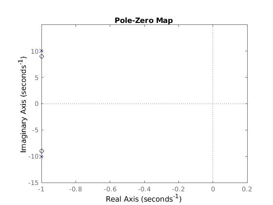
poles = [-1+10j,-1-10j];

zeroes = [-1-9j,-1+9j];

z = poly(zeroes);

p = poly(poles);

Hs1 = tf(z,p);

pzmap(Hs1,'b')

x = bodeoptions;

x.XLim = [0.1 100];

figure(1)

bode(Hs1,x)

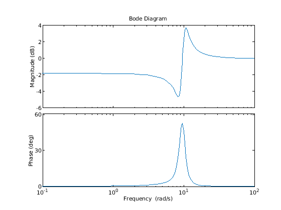
man sieht: die Nullstelle neutralisiert die nahe Polstelle, der zusätzliche Pol überwiegt, bei w=3 ist die Phase -45°; dann aber kommt man in einen Frequenzbereich, in dem zuerst die Nulllstelle, dann der Pol eine kleine Abweichung erzeugen; ist der Abstand von diesen beiden Punkten groß genug, wirkt wieder nur der eine Pol und dreht die Phase auf -90*

Eingabe: Übertragungsfunktion in s

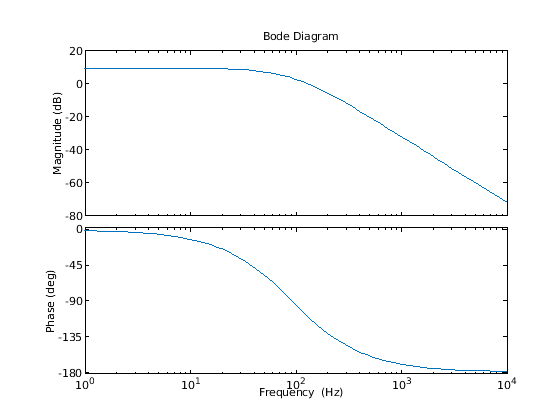
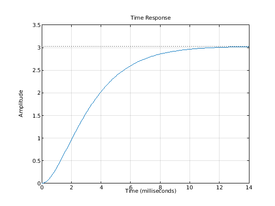
PT2 Glied

s=tf("s");

G3=(1e6)/((s+550)*(s+600));

g=bodeoptions;

%g.MagUnits = 'abs';

%g.FreqScale='linear';

g.FreqUnits='Hz';

bodeplot(G3,g);

p=timeoptions;

p.TimeUnits = 'milliseconds';

stepplot(G3,p)

grid on

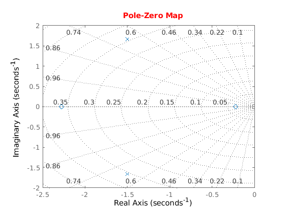
Eingabe: Polynome

 

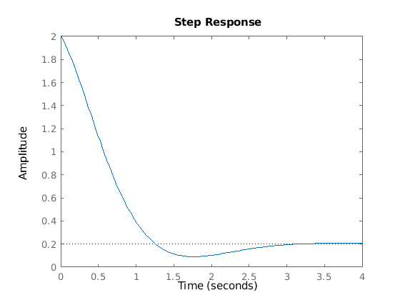
sys = tf([2 5 1],[1 3 5]);

h = pzplot(sys);

grid on

p = getoptions(h);

p.FreqUnits = 'Hz';

p.Title.Color = [1,0,0];

setoptions(h,p);

g=bodeoptions;

g.MagUnits = 'abs';

g.FreqScale='linear';

q.FreqUnits='Hz';

bodeplot(sys,g);

stepplot(sys)